1. Introduction: The Double-Edged Sword of Decision Trees
Decision trees are among the most commonly used algorithms in machine learning, highly valued for their clarity and straightforward implementation. At their core, they function by recursively splitting data based on the most informative feature, resulting in a branching, tree-like structure. This logical flow of decisions makes the model exceptionally easy to interpret, which is crucial in fields like healthcare or finance where transparency is demanded.
However, despite their advantages, decision trees are prone to becoming overly complex. If allowed to grow without constraints, a tree may start to memorize the training data—including its inherent noise and random outliers—rather than learning the broad, generalizable patterns. This phenomenon is known as overfitting. An overfitted tree will demonstrate exceptionally high accuracy on its training data but will perform poorly on unseen datasets. To build robust learning systems, we must move beyond the basic algorithm and apply advanced techniques to control complexity, handle messy real-world data, and optimize performance.
2. The Mechanics of Overfitting and the Bias-Variance Tradeoff
A decision tree overfits when it grows too deep, capturing very detailed rules that apply exclusively to the specific training dataset. Because the algorithm's goal is to minimize error on the training set, it might create branches based on minute, insignificant differences in the data.
Imagine we are building a decision tree to determine whether a customer will purchase a product. If the tree becomes too complex, it might generate a highly specific rule like: "Predict 'yes' if the customer is 22 years old, earns $35,000, and viewed a particular product three times". This rule is too tailored to the training examples and will likely fail to generalize to new customers with slightly different characteristics.
Overfitting is intimately tied to the bias-variance tradeoff.
Bias is the error that occurs when a model makes overly simple assumptions about the data, leading to underfitting.
Variance is the error that occurs when a model is too sensitive to the training data, capturing random fluctuations and noise.
An overfitted decision tree typically exhibits low bias but suffers from incredibly high variance. The objective in advanced tree building is to achieve a balance: capturing important patterns without getting distracted by noise.
3. Taming the Tree: Powerful Pruning Techniques
To maintain the right balance and prevent overfitting, data scientists use techniques known as pruning to simplify the tree. Pruning involves removing sections of the tree that add little predictive value, thereby enhancing its ability to generalize.
Pre-Pruning (Early Stopping) Pre-pruning involves placing strict restrictions on the tree’s growth during the actual training phase. Techniques include setting a maximum depth for the tree (e.g., allowing no more than 5 levels of splits) or requiring a minimum number of samples per leaf (e.g., forcing the tree to stop splitting if a node has fewer than 10 data points). This forces the model to focus on broader, more meaningful trends.
Reduced Error Pruning (REP) Reduced Error Pruning is a post-training method. First, the decision tree is allowed to grow fully. Then, a separate "validation dataset" (data not used during training) is used to evaluate the model's performance. The algorithm systematically focuses on each branch and checks if removing it would improve or maintain the tree's performance on the validation set. If performance improves or remains unchanged, the branch is permanently pruned. This results in a smaller, more robust tree that is less sensitive to small variations in training data.
Rule Post Pruning Rule post pruning is another highly effective technique. After the tree is fully grown, every single path from the root node to a leaf node is translated into a sequence of "IF-THEN" rules. For instance, a rule might be: "If age > 60 and blood pressure > 140, then predict disease". Each individual rule is then evaluated against a validation dataset to see how much it contributes to overall accuracy. Rules or conditions that offer no benefit are eliminated. This method is highly favored because removing redundant rules drastically improves the interpretability and readability of the model for human stakeholders.
4. Handling Real-World Data Complexities
Standard decision tree tutorials often use clean, categorical data. However, real-world data is messy, continuous, and frequently missing.
Incorporating Continuous-Valued Attributes While categorical variables (like "Red" or "Blue") are easy to split, continuous variables (like age, income, or temperature) require the tree to find optimal mathematical thresholds. The algorithm handles this by first sorting the continuous data in ascending or descending order. It then tests various potential split points (thresholds) between the data points. For example, if analyzing income, the tree will evaluate different thresholds and calculate the resulting impurity—using metrics like Gini Impurity or Entropy—for each potential split. The threshold that results in the greatest reduction of impurity (the best separation of classes) is selected as the decision boundary for that node.
Handling Missing Attribute Values Missing data can severely hinder a decision tree's ability to make accurate splits. Advanced implementations address this using several strategies:
Mean/Median/Mode Imputation: A straightforward approach is to replace missing numerical values with the dataset's mean or median, and missing categorical values with the most frequent category (mode).
Surrogate Splits: When a key attribute is missing for a specific data point, the algorithm can use a "surrogate split"—an alternative feature that acts as a backup. For instance, if "age" is missing but is highly correlated with "income", the tree might use the income feature to determine which path the data point should take.
Data Imputation (e.g., KNN): More complex methods use algorithms like K-Nearest Neighbors to predict and fill in the missing value based on the patterns of similar instances in the dataset.
Cost-Sensitive Decision Making In business and healthcare, not all data is equally easy or cheap to acquire. Extracting a patient's age is essentially free, but running a specialized blood test costs money. Cost-sensitive decision trees adjust the tree-building process to account for the relative financial or computational costs of different attributes. By assigning a "weight" or "cost factor" to each feature, the algorithm evaluates splits based on a cost-adjusted gain. If a cheap feature (like income) provides similar predictive power to an expensive feature (like a third-party credit score check), the tree will prioritize splitting on the cheaper feature. This makes the resulting model highly efficient for real-world deployment.
5. Supercharging Trees: Ensemble Methods
While a single decision tree is interpretable, it is often not the most powerful predictive model due to its high variance. To achieve state-of-the-art accuracy, data scientists turn to Ensemble Methods, which combine the predictions of multiple decision trees.
Bagging (Bootstrap Aggregating) Bagging aims to reduce the variance of a model, making it less prone to overfitting. It works by randomly sampling the training data with replacement to create multiple "bootstrap samples". A separate, independent decision tree is trained on each sample. Because they are trained on slightly different data, they learn different decision boundaries. When a new prediction is required, the outputs of all the trees are aggregated—typically by majority voting for classification or averaging for regression. Random Forest is a famous implementation of bagging that further introduces randomness by restricting the features each tree can evaluate.
Boosting Unlike Bagging, which trains trees independently and in parallel, Boosting trains a series of "weak learners" (usually very shallow decision trees) sequentially. Each new tree is specifically trained to correct the residual errors made by the previous trees. Boosting places heavier mathematical weights on the data points that were misclassified in previous iterations, forcing the algorithm to focus intensely on hard-to-predict examples. The final prediction is a weighted sum of all the sequential trees. While Bagging primarily reduces variance, Boosting is highly effective at reducing model bias.
Conclusion
Decision trees represent a foundational pillar of machine learning, but deploying them effectively requires moving beyond the basic algorithms. By understanding the dangers of overfitting and actively combating it with pre-pruning, Reduced Error Pruning, and Rule Post Pruning, we can create models that generalize reliably to unseen data. Furthermore, by equipping our models to handle continuous thresholds, missing values, and varying data collection costs, we transition decision trees from theoretical exercises into robust, cost-effective business tools. Finally, by integrating them into powerful ensemble methods like Random Forests and Gradient Boosting, decision trees continue to drive some of the most accurate predictive systems in the world today.